Advanced Tutorial 3 : build a Spectral Deferred Correction solver for non-linear ODEs

📜 Previous base tutorial onSDCfocused on the Dahlquist problem to explain how to use the \(Q_\Delta\)-coefficients. But we can also use those for non-linear ODEsas long as \(Q_\Delta\) is lower triangular.

Back to the all-at-once system defined for the previous tutorial :

\[{\bf u} - \Delta{t}Q {\bf f} = {\bf u}_0,\]

with \(Q\) a dense matrix. We still want to be able to solve this system using only :

• evaluation of \(f(u,t)\)

• solution of \(u-\alpha f(u,t) = rhs\) for any \(\alpha,t,rhs\)

Then, we consider the preconditioned iteration to solve the all-at-once system :

\[(I - \Delta{t}Q_\Delta F)({\bf u}^{k+1} - {\bf u}^{k}) = {\bf u}_0 - ({\bf u}^{k} - \Delta{t}Q {\bf f}^{k})\]

where \({\bf u}^{k} := [u_1^k, \dots, u_M^k]^T\) the vector of node solutions at the \(k^{th}\) iteration and \({\bf f}^{k} := [f(u_1^k, t_1), \dots, f(u_M^k, t_M)]^T\) the evaluation of each node solution. We use the notation \(I,F\) for the identity operator and \(f\) evaluation, respectively.

The iteration can be rewritten and simplified into

\[{\bf u}^{k+1} - \Delta{t}Q_\Delta {\bf f}^{k+1} = {\bf u}_0 + \Delta{t}(Q-Q_\Delta) {\bf f}^{k}\]

which can be solved node by node for each iteration, as long as \(Q_\Delta\) is lower triangular.

Prerequisite

We use the same as for the previous tutorial :

import numpy as np
from scipy.optimize import fsolve

u0 = np.array([5, -5, 20])
sigma, rho0, beta, epsilon = 10, 28, 8/3, 5


def f(u, t):
    x, y, z = u
    rho = rho0 + epsilon*np.sin(t)
    return np.array([sigma*(y-x), x*(rho-z)-y, x*y-beta*z])


def fSolve(a, t, rhs, uInit):

    def res(u):
        return u - a*f(u, t) - rhs

    return fsolve(res, uInit)

Implementation

Let’s retrieve \(Q\) and \(Q_\Delta\) coefficients fom qmat, using the Collocation class as base

from qmat.qcoeff.collocation import Collocation
from qmat import genQDeltaCoeffs

qGen = Collocation(nNodes=4, nodeType="LEGENDRE", quadType="RADAU-RIGHT")
nodes, weights, Q = qGen.genCoeffs()
QDelta = genQDeltaCoeffs("BE", qGen=qGen)

📜 Checkout the tutorial on nodes generation for details about nodeType and quadType.

Then we define some arrays to store the node solutions for each iterations (considering here \(K=4\) sweeps), the step solutions and time values :

nSweeps = 4
uNodes = np.zeros((nSweeps+1, nodes.size, u0.size))     # k=0,...,K => (nSweeps+1) node solutions vectors

tEnd = 10
nSteps = 1000

uNum = np.zeros((nSteps+1, u0.size))
times = np.linspace(0, tEnd, nSteps+1)

Now, for each time step, time node and iteration, we have to solve

\[u_m^{k+1} - \Delta{t} q^\Delta_{m,m} f(u_m^{k+1},t_m) = u_0 + \Delta{t} \sum_{j=1}^{M} q_{m,j}f(u_j^{k},t_j) + \Delta{t} \sum_{j=1}^{m-1} q^\Delta_{m,j}f(u_j^{k+1},t_j) - \Delta{t} \sum_{j=1}^{m} q^\Delta_{m,j}f(u_j^{k},t_j)\]

and compute the step update before next step :

\[u(t_0 + \Delta{t}) \simeq u_0 + \sum_{m=1}^{M} \omega_{m} f(u_m, t_m).\]

This can be done with the following code :

uNum[0] = u0
for i in range(nSteps):
    dt = times[i+1] - times[i]
    tNodes = times[i] + dt*nodes

    # Initialize k=0 with u0
    uNodes[0][:] = uNum[i]

    # Iteration loop
    for k in range(nSweeps):

        # Loop on nodes
        for m in range(len(nodes)):
            rhs = uNum[i].copy()

            # Quadrature terms
            for j in range(len(nodes)):
                rhs += dt*Q[m, j]*f(uNodes[k, j], tNodes[j])

            # Correction terms
            for j in range(m):
                rhs += dt*QDelta[m, j]*f(uNodes[k+1, j], tNodes[j])
            for j in range(m+1):
                rhs -= dt*QDelta[m, j]*f(uNodes[k, j], tNodes[j])

            if QDelta[m,m] == 0:
                uNodes[k+1, m] = rhs
            else:
                uNodes[k+1, m] = fSolve(dt*QDelta[m, m], tNodes[m], rhs, uInit=uNodes[k, m])

    # Step update
    uNum[i+1] = uNum[i]
    for m in range(len(nodes)):
        uNum[i+1] += dt*weights[m]*f(uNodes[-1, m], tNodes[m])

And that’s it 🥳 ! We solved our non-linear time-dependent ODE on the given time frame using 4 SDC sweeps, without caring about what’s in our \(Q\) and \(Q_\Delta\) coefficients …

🔍 For a strictly lower triangular \(Q_\Delta\) matrix (QDelta[m,m]=0), there is no need for the fSolve function (as for the RK methods in previous tutorial). We talk then about explicit SDC sweeps.

💡 Here the same \(Q_\Delta\) matrix is used for all sweeps, but nothing prevent to use different \(Q_\Delta\) coefficient for each different sweeps. We just have to generate a \(Q_\Delta\) matrix with shape (nSweeps, nNodes, nNodes), which is allowed using the nSweeps optional parameter of genQDeltaCoeffs.

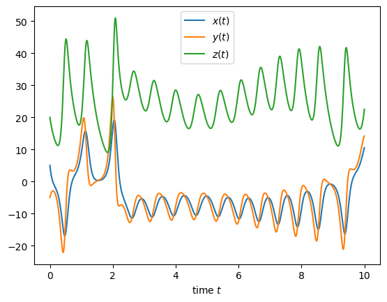
Finally, we can plot the solution with respect to time :

import matplotlib.pyplot as plt

plt.plot(times, uNum[:, 0], label="$x(t)$")
plt.plot(times, uNum[:, 1], label="$y(t)$")
plt.plot(times, uNum[:, 2], label="$z(t)$")
plt.legend(); plt.xlabel("time $t$");

Ideally, the previous code can be written into a function to allow multiple calls :

def solveSDC(nSteps, nSweeps, scheme):
    qGen = Collocation(nNodes=4, nodeType="LEGENDRE", quadType="RADAU-RIGHT")
    nodes, weights, Q = qGen.genCoeffs()
    QDelta = genQDeltaCoeffs(scheme, qGen=qGen)

    uNodes = np.zeros((nSweeps+1, nodes.size, u0.size))

    tEnd = 10
    uNum = np.zeros((nSteps+1, u0.size))
    times = np.linspace(0, tEnd, nSteps+1)

    uNum[0] = u0
    for i in range(nSteps):
        dt = times[i+1] - times[i]
        tNodes = times[i] + dt*nodes

        # Initialize k=0 with u0
        uNodes[0][:] = uNum[i]

        # Iteration loop
        for k in range(nSweeps):

            # Loop on nodes
            for m in range(len(nodes)):
                rhs = uNum[i].copy()

                # Quadrature terms
                for j in range(len(nodes)):
                    rhs += dt*Q[m, j]*f(uNodes[k, j], tNodes[j])

                # Correction terms
                for j in range(m):
                    rhs += dt*QDelta[m, j]*f(uNodes[k+1, j], tNodes[j])
                for j in range(m+1):
                    rhs -= dt*QDelta[m, j]*f(uNodes[k, j], tNodes[j])

                if QDelta[m,m] == 0:
                    uNodes[k+1, m] = rhs
                else:
                    uNodes[k+1, m] = fSolve(dt*QDelta[m, m], tNodes[m], rhs, uInit=uNodes[k, m])

        # Step update
        uNum[i+1] = uNum[i]
        for m in range(len(nodes)):
            uNum[i+1] += dt*weights[m]*f(uNodes[-1, m], tNodes[m])

    return times, uNum

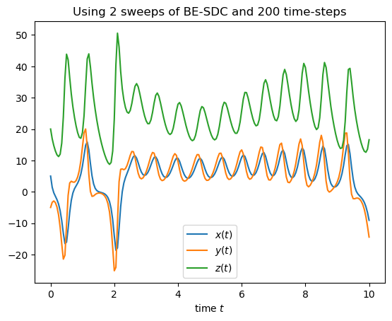
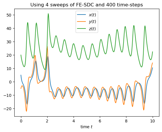
… which can be used to try different SDC schemes, number of sweeps or time resolution :

times, uNum = solveSDC(200, 2, "BE")
plt.plot(times, uNum[:, 0], label="$x(t)$")
plt.plot(times, uNum[:, 1], label="$y(t)$")
plt.plot(times, uNum[:, 2], label="$z(t)$")
plt.legend(); plt.xlabel("time $t$"); plt.title("Using 2 sweeps of BE-SDC and 200 time-steps");

times, uNum = solveSDC(400, 4, "FE")
plt.plot(times, uNum[:, 0], label="$x(t)$")
plt.plot(times, uNum[:, 1], label="$y(t)$")
plt.plot(times, uNum[:, 2], label="$z(t)$")
plt.legend(); plt.xlabel("time $t$"); plt.title("Using 4 sweeps of FE-SDC and 400 time-steps");

Using the internal SDC solver

Such generic SDC solver is also available in the qmat.solvers.generic.CoeffSolver class, and uses a more efficient implementation than the one showed above, requiring less evaluation of \(f(u,t)\). This implementation is based on the DiffOp class that implements the \(f(u,t)\) evaluations, see the last part of the previous tutorial for more details.

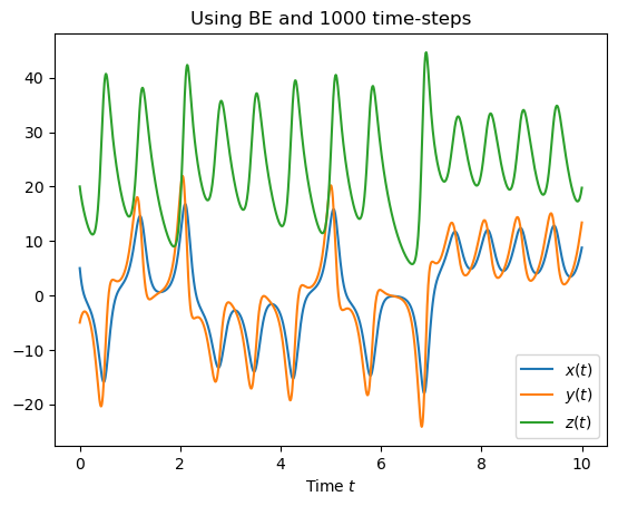
Looking at the non-perturbed Lorenz example problem, we can solve it with SDC using those few lines :

from qmat import genQDeltaCoeffs
from qmat.qcoeff.collocation import Collocation
from qmat.solvers.generic import CoeffSolver
from qmat.solvers.generic.diffops import Lorenz

scheme = "BE"
nSteps = 1000
nSweeps = 4

qGen = Collocation(nNodes=4, nodeType="LEGENDRE", quadType="RADAU-RIGHT")
nodes, weights, Q = qGen.genCoeffs()
QDelta = genQDeltaCoeffs(scheme, qGen=qGen)

solver = CoeffSolver(Lorenz(), tEnd=10, nSteps=nSteps)
uNum = solver.solveSDC(nSweeps, Q, weights, QDelta)

plt.plot(solver.times, uNum[:, 0], label="$x(t)$")
plt.plot(solver.times, uNum[:, 1], label="$y(t)$")
plt.plot(solver.times, uNum[:, 2], label="$z(t)$")
plt.legend(); plt.xlabel("Time $t$"); plt.title(f"Using {scheme} and {nSteps} time-steps");

Eventually, you can also add your own differential operator into qmat, see the short developer guide on this aspect …

💡 This coefficient-based approach for SDC, relying on a \(Q_\Delta\) matrix, allows many different variants by just changing the \(Q_\Delta\) coefficients. However, it always relies on multi-node (or multi-stage) methods to define the approximate time-integrator used for the SDC sweeps.

But one can also define SDC in an even more generic way, using a \(\phi\)-based representation of time integrators, which is the topic of the next tutorial.