Advanced Tutorial 2 : build a Runge-Kutta solver for non-linear ODEs

📜 Previous base tutorial onRunge-Kutta solverfocused on the Dahlquist problem to explain how to use the \(Q\)-coefficients. But we can also use those for non-linear ODEsas long as \(Q\) is lower triangular.

Consider the following (non-linear) ODE system :

\[\frac{du}{dt}= f(u,t), \quad u(t_0)=u_0,\]

where \(t_0\) is the initial time. Computing the solution after one time-step \(u(t_0+\Delta)\) using the \(Q\)-coefficients (or Butcher table) or size \(M\) :

\[\begin{split}\begin{array} {c|c} \tau & Q \\ \hline & w^\top \end{array}\end{split}\]

corresponds to approximating the solution at time nodes (or stages) \([t_1, \dots, t_M] := [t_0+\Delta{t}\tau_1, \dots, t_0+\Delta{t}\tau_M]\) by solving the all-at-once system :

\[{\bf u} - \Delta{t}Q {\bf f} = {\bf u}_0 \quad (1)\]

where \({\bf u} := [u_1,\dots,u_M]^T\) is the vector containing the node solutions (or stages), \({\bf f} := [f(u_1, t_1),\dots,f(u_M,t_M)]^T\) the evaluations of each node solutions and \({\bf u}_0\) a vector with \(u_0\) in each of its entries.

Then, \(u(t_0+\Delta{t})\) can be approximated via the step update :

\[u(t_0+\Delta{t}) \simeq u_0 + \sum_{m=1}^{M} \omega_{m} f(u_m, t_m) \quad (2)\]

and this process can be repeated for each successive time-step.

📣 If we do not want to solve \((1)\) all-at-once (which can be very expensive for large problem), then \(Q\) must be lower-triangular to allow forward substitution, i.e solve for \(u_1\) first, then for \(u_2\) using the \(u_1\) solution, etc …

Prerequisite

Consider for example the perturbed Lorenz attractor :

\[\begin{split}\begin{align} \frac{dx}{dt} &= \sigma(y-x) \\ \frac{dy}{dy} &= x(\rho(t)-z) - y, \quad \rho(t) = \rho_0 + \epsilon \sin(t) \\ \frac{dz}{dt} &= xy - \beta z \end{align}\end{split}\]

Before solving it, we first need to define its differential operator \(f(u, t)\) with \(u=[x,y,z]^T\) and the associated initial solution \(u_0\) for our problem :

import numpy as np

u0 = np.array([5, -5, 20])
sigma, rho0, beta, epsilon = 10, 28, 8/3, 5

def f(u, t):
    x, y, z = u
    rho = rho0 + epsilon*np.sin(t)
    return np.array([sigma*(y-x), x*(rho-z)-y, x*y-beta*z])

In addition, if we want to use an implicit method, we need to define a fSolve function that solves

\[u - \alpha f(u, t) = rhs\]

for any \(\alpha\) and \(rhs\), using some uInit parameter as initial guess. To simplify, we can quickly implement one using the fsolve function of scipy.optimize (interface for MINPACK) :

from scipy.optimize import fsolve

def fSolve(a, t, rhs, uInit):

    def res(u):
        return u - a*f(u, t) - rhs

    return fsolve(res, uInit)

Implementation

Let’s retrieve some \(Q\) coefficients from qmat :

from qmat import genQCoeffs
nodes, weights, Q = genQCoeffs("DIRK43")    # Implicit RK method of order three in 4 stages

and define some arrays to store the node solutions, the step solutions and time values :

uNodes = np.zeros((nodes.size, u0.size))

tEnd = 10
nSteps = 1000

uNum = np.zeros((nSteps+1, u0.size))
times = np.linspace(0, tEnd, nSteps+1)

Now, for each time step and time node, we have to solve

\[u_{m} - \Delta{t}q_{m,m}f(u_m,t_m) = u_0 + \Delta{t}\sum_{j=1}^{m-1}q_{m,j}f(u_j, t_j),\]

and compute the step update before next time-step :

\[u(t_0+\Delta{t}) \simeq u_0 + \sum_{m=1}^{M} \omega_{m} f(u_m, t_m).\]

This can be done with the following code :

uNum[0] = u0
for i in range(nSteps):
    dt = times[i+1] - times[i]
    tNodes = times[i] + dt*nodes

    # Solve for each time nodes (stages)
    for m in range(len(nodes)):
        rhs = uNum[i].copy()

        for j in range(m):
            rhs += dt*Q[m, j]*f(uNodes[j], tNodes[j])

        if Q[m,m] == 0:
            uNodes[m] = rhs
        else:
            uNodes[m] = fSolve(dt*Q[m, m], tNodes[m], rhs, uInit=uNum[i])

    # Step update
    uNum[i+1] = uNum[i]
    for m in range(len(nodes)):
        uNum[i+1] += dt*weights[m]*f(uNodes[m], tNodes[m])

And that’s it 🥳 ! We solved our non-linear time-dependent ODE on the given time frame, without caring about what’s in our \(Q\)-coefficients …

🔍 For a strictly lower triangular \(Q\) matrix (Q[m,m]=0), there is no need for the fSolve function, as the solution is simply \(rhs\). That’s the case for all explicit Runge-Kutta methods.

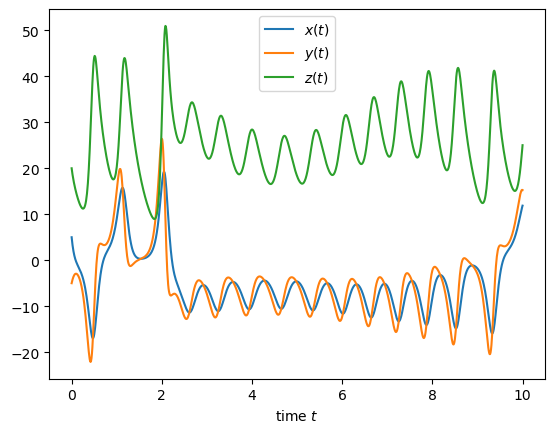
We can plot the solution with respect to time :

import matplotlib.pyplot as plt

plt.plot(times, uNum[:, 0], label="$x(t)$")
plt.plot(times, uNum[:, 1], label="$y(t)$")
plt.plot(times, uNum[:, 2], label="$z(t)$")
plt.legend(); plt.xlabel("time $t$");

Ideally, the previous code can be written into a function to allow multiple calls :

def solve(nSteps, scheme):

    nodes, weights, Q = genQCoeffs(scheme)
    uNodes = np.zeros((nodes.size, u0.size))

    uNum = np.zeros((nSteps+1, u0.size))
    times = np.linspace(0, tEnd, nSteps+1)

    uNum[0] = u0
    for i in range(nSteps):
        dt = times[i+1] - times[i]
        tNodes = times[i] + dt*nodes

        # Solve for each time nodes (stages)
        for m in range(len(nodes)):
            rhs = uNum[i].copy()

            for j in range(m):
                rhs += dt*Q[m, j]*f(uNodes[j], tNodes[j])

            if Q[m,m] == 0:
                uNodes[m] = rhs
            else:
                uNodes[m] = fSolve(dt*Q[m, m], tNodes[m], rhs, uInit=uNum[i])

        # Step update
        uNum[i+1] = uNum[i]
        for m in range(len(nodes)):
            uNum[i+1] += dt*weights[m]*f(uNodes[m], tNodes[m])

    return times, uNum

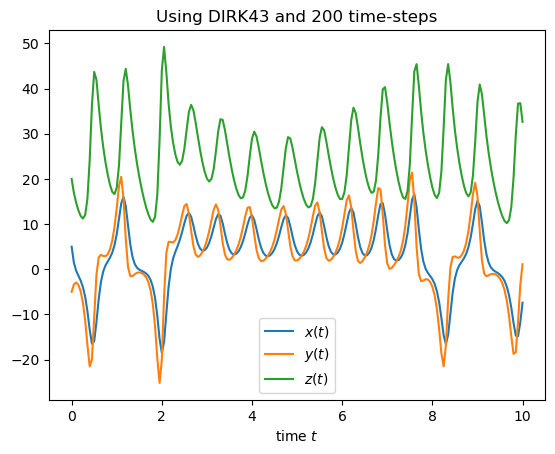
… which can be used to try different time schemes or resolution :

times, uNum = solve(200, "DIRK43")
plt.plot(times, uNum[:, 0], label="$x(t)$")
plt.plot(times, uNum[:, 1], label="$y(t)$")
plt.plot(times, uNum[:, 2], label="$z(t)$")
plt.legend(); plt.xlabel("time $t$"); plt.title("Using DIRK43 and 200 time-steps");

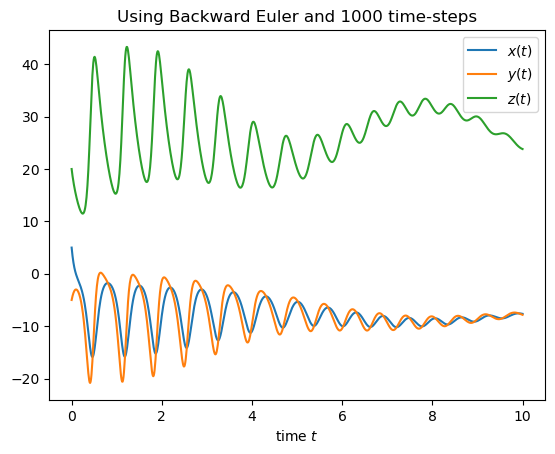
times, uNum = solve(1000, "BE")
plt.plot(times, uNum[:, 0], label="$x(t)$")
plt.plot(times, uNum[:, 1], label="$y(t)$")
plt.plot(times, uNum[:, 2], label="$z(t)$")
plt.legend(); plt.xlabel("time $t$"); plt.title("Using Backward Euler and 1000 time-steps");

Using the internal RK solver

Such generic Runge-Kutta solver is also available in qmat in the qmat.solvers.generic.CoeffSolver class, and uses a more efficient implementation than the one showed above, requiring less evaluations of \(f(u,t)\).

This implementation is based on a DiffOp class (differential operator) that implements the \(f(u,t)\) evaluation using the following template :

from qmat.solvers.generic import DiffOp

class Yoodlidoo(DiffOp):
    def __init__(self, params="value"):
        # use some initialization parameters
        u0 = ... # define your initial vector
        super().__init__(u0)

    def evalF(self, u, t, out:np.ndarray):
        r"""
        Evaluate :math:`f(u,t)` and store the result into `out`.

        Parameters
        ----------
        u : np.ndarray
            Input solution for the evaluation.
        t : float
            Time for the evaluation.
        out : np.ndarray
            Output array in which is stored the evaluation.
        """
        out[:] = ... # put the result into out

Note that the evalF function does not return the result, but rather put the result of the evaluation into the out array. This allows a memory efficient implementation of the different solvers that avoids any implicit data copy.

🔔 The DiffOp base class also provide a default fSolve method, so you don’t need to implement it.

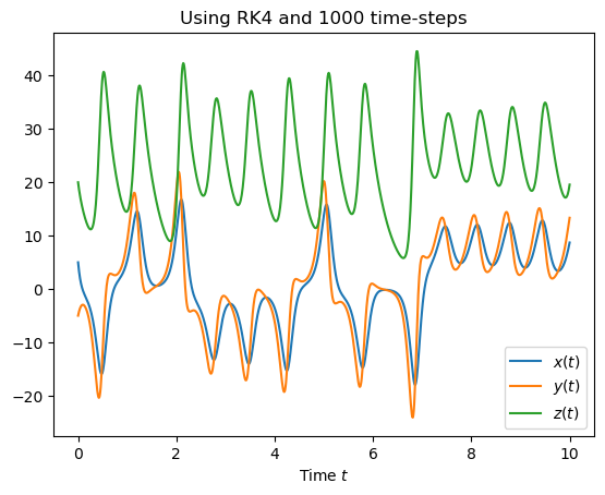
Some differential operators are already provided in qmat … for example, to solve the non-perturbed Lorenz system using a Runge-Kutta approach :

from qmat import genQCoeffs
from qmat.solvers.generic import CoeffSolver
from qmat.solvers.generic.diffops import Lorenz

scheme = "RK4"
nSteps = 1000

solver = CoeffSolver(Lorenz(), tEnd=10, nSteps=nSteps)

nodes, weights, Q = genQCoeffs(scheme)
uNum = solver.solve(Q, weights)

plt.plot(solver.times, uNum[:, 0], label="$x(t)$")
plt.plot(solver.times, uNum[:, 1], label="$y(t)$")
plt.plot(solver.times, uNum[:, 2], label="$z(t)$")
plt.legend(); plt.xlabel("Time $t$"); plt.title(f"Using {scheme} and {nSteps} time-steps");

Eventually, you can also add your own differential operator into qmat, see the short developer guide on this aspect …

📣 This Runge-Kutta solver does not work if \(Q\) is a dense matrix. In that case, we can eventually use the Spectral Deferred Correction approach without too much additional code, which is the topic of the next advanced tutorial …