Advanced Tutorial 4 : build a Spectral Deferred Correction solver based on generic time-integrators
📜 Previous advanced tutorial onSDCfocused on its implementation for non-linear ODEs using \(Q_\Delta\)-coefficients. But we can also define a SDC sweepwithout \(Q_\Delta\) coefficients, and extend this idea to many other time-integration approaches.
©️ Credits to Martin Schreiber for the original idea.
\(\phi\)-based time-integrator :
Considering a sequence of nodes \(\{\tau_1, ..., \tau_M\}\) discretizing one time-step \(\{t_0, t_0+\Delta{t}\}\) into \(\{t_1, \dots, t_M\} := \{t_0+\Delta{t}\tau_1, \dots, t_0 + \Delta{t}\tau_M\}\). We can write one time-integrator computing the step solution through all node as a \(\phi\) function such that :
This allows to represent any time-integrator, without writing it in a \(Q\)-coefficient framework. In particular, if we look at the Picard form of an ODE written at a given time node :
the \(\phi\) function simply corresponds to a given discretization of the integral into the time nodes \(\{t_1, \dots, t_m\}\), with no dependency to the next time nodes.
Continuous Spectral Deferred Correction
To retrieve the original SDC formulation of SDC, we define the error \(e^{k}(t) = u(t) - u^{k}(t)\) and put it in the Picard equation above to get :
Noting \(u^{k+1}(t) := e^{k}(t) + u^{k}(t)\) and adding the difference of the two same integral terms with \(u^{k}\) we get :
\(\phi\)-based Spectral Deferred Correction :
We write the continuous SDC equation at a given time node \(t_{m+1}\), use a given \(\phi\) time integrator to replace the first two integrals, and write the last integral using a quadrature rule on all time nodes :
or in final form :
✨ And there it is : no need of any \(Q_\Delta\) coefficient ! We just need to use the definition of a time-integrator that allows to
evaluate \(\phi(u_0, u_1, ..., u_{m+1})\) for any sequences of node solutions up to the \((m+1)^{th}\) one,
solve \(u - \phi(u_0, u_1, ..., u_{m}, u) = rhs\) for any \(rhs\) vector.
Prerequisite
We use the same as for the previous tutorial :
[1]:
import numpy as np
from scipy.optimize import fsolve

u0 = np.array([5, -5, 20])
sigma, rho0, beta, epsilon = 10, 28, 8/3, 5


def f(u, t):
    x, y, z = u
    rho = rho0 + epsilon*np.sin(t)
    return np.array([sigma*(y-x), x*(rho-z)-y, x*y-beta*z])


def fSolve(a, t, rhs, uInit):

    def res(u):
        return u - a*f(u, t) - rhs

    return fsolve(res, uInit)
In addition, we define our underlying collocation problem :
[2]:
from qmat.qcoeff.collocation import Collocation

qGen = Collocation(nNodes=4, nodeType="LEGENDRE", quadType="RADAU-RIGHT")
nodes, weights, Q = qGen.genCoeffs()
Implementation
Consider a Backward Euler step between each node, and let us write it in \(\phi\) formulation. Defining \(\Delta{\tau}_m = t_{m}-t_{m-1}\), we have for each node
By substitution we can rearrange those into :
so we can identify the \(\phi\) function for Backward Euler :
[3]:
def phi(uNodes, t0, dt):
    tau = [t0] + (t0 + dt*nodes).tolist()
    out = 0
    for i, u in enumerate(uNodes[1:]):
        dTau = tau[i+1] - tau[i]
        out = out + dTau*f(u, tau[i+1])
    return out
Then we can define a function to solve \(u - \phi(u_0, u_1, ..., u_{m}, u) = rhs\) for any \(rhs\) vector :
[4]:
from scipy.optimize import fsolve

def phiSolve(uNodes, rhs, uInit, t0, dt):
    tau = [t0] + (t0 + dt*nodes).tolist()

    for i, u in enumerate(uNodes[1:]):
        dTau = tau[i+1] - tau[i]
        rhs = rhs + dTau*f(u, tau[i+1])

    m = len(uNodes) - 1
    dTau = tau[m+1] - tau[m]
    def res(u):
        return u - dTau*f(u, tau[m+1]) - rhs

    return fsolve(res, uInit)
And now, we just need to implement the \(\phi\)-based SDC formula as defined before :
[5]:
nSweeps = 4
uNodes = np.zeros((nSweeps+1, nodes.size, u0.size))

tEnd = 10
nSteps = 1000

uNum = np.zeros((nSteps+1, u0.size))
times = np.linspace(0, tEnd, nSteps+1)


uNum[0] = u0
for i in range(nSteps):
    dt = times[i+1] - times[i]
    tNodes = times[i] + dt*nodes
    u0 = uNum[i]

    # Initialize k=0 with u0
    uNodes[0][:] = u0

    # Iteration loop
    for k in range(nSweeps):

        # Loop on nodes
        for m in range(len(nodes)):
            rhs = uNum[i].copy()

            # Quadrature terms
            for j in range(len(nodes)):
                rhs += dt*Q[m, j]*f(uNodes[k, j], tNodes[j])

            # Phi correction term
            rhs -= phi([u0, *uNodes[k, :m+1]], times[i], dt)

            # Phi solve
            uNodes[k+1, m] = phiSolve([u0, *uNodes[k+1, :m]], rhs, uNodes[k, m], times[i], dt)

    # Step update
    uNum[i+1] = u0
    for m in range(len(nodes)):
        uNum[i+1] += dt*weights[m]*f(uNodes[-1, m], tNodes[m])
And that’s it 🥳 ! We solved our non-linear time-dependent ODE on the given time frame using 4 SDC sweeps, without using any \(Q_\Delta\) coefficients …
As before, we can plot the solution with respect to time :
[6]:
import matplotlib.pyplot as plt

plt.plot(times, uNum[:, 0], label="$x(t)$")
plt.plot(times, uNum[:, 1], label="$y(t)$")
plt.plot(times, uNum[:, 2], label="$z(t)$")
plt.legend(); plt.xlabel("time $t$");
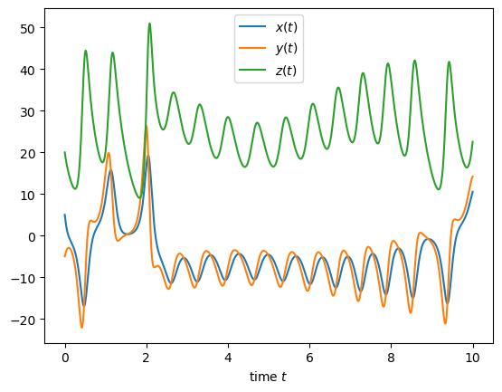
💡 Note that we retrieve exactly the same solution as the first application example given in previous tutorial.
And as before, we can implement a function to reuse it with different time resolution, blablabla …
Using the internal \(\phi\)-SDC solver
An optimized implementation of this \(\phi\)-SDC approach is implemented in the qmat.solvers.generic.PhiSolver class, along with some classical time integrator written in \(\phi\) formulation. As for the CoeffSolver used in previous tutorials, they use a DiffOp class to evaluate \(f(u,t)\).
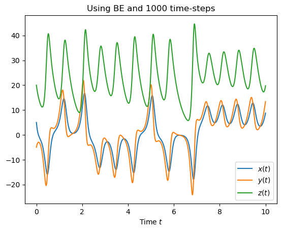
Looking at the non-perturbed Lorenz example problem (again), we can solve it with \(\phi\)-SDC using those few lines :
[7]:
from qmat.qcoeff.collocation import Collocation
from qmat.solvers.generic.integrators import BackwardEuler
from qmat.solvers.generic.diffops import Lorenz

scheme = "BE"
nSteps = 1000
nSweeps = 4

qGen = Collocation(nNodes=4, nodeType="LEGENDRE", quadType="RADAU-RIGHT")
nodes, weights, Q = qGen.genCoeffs()

solver = BackwardEuler(Lorenz(), nodes, tEnd=10, nSteps=nSteps)
uNum = solver.solveSDC(nSweeps, Q, weights)

plt.plot(solver.times, uNum[:, 0], label="$x(t)$")
plt.plot(solver.times, uNum[:, 1], label="$y(t)$")
plt.plot(solver.times, uNum[:, 2], label="$z(t)$")
plt.legend(); plt.xlabel("Time $t$"); plt.title(f"Using {scheme} and {nSteps} time-steps");
📣 Additional \(\phi\) integrators can be implemented, using the following template :
[8]:
from qmat.solvers.generic import PhiSolver

class Phidlidoo(PhiSolver):

    def evalPhi(self, uVals, fEvals, out, t0=0):
        """
        Parameters
        ----------
        uVals : list[np.ndarray] of size :math:`m+2`
            The :math:`m+1` time-node solutions + the initial solution :math:`u_0`.
        fEvals : list[np.ndarray] of size :math:`m+1` or :math:`m+1`
            The :math:`f(u,t)` evaluations at each time nodes (+ initial solution),
            up to time-node :math:`m`.
            It can eventually contain a pre-computed :math:`f_{m+1}`
            to spare one :math:`f(u,t)` evaluation.
        out : np.ndarray
            Array used to store the evaluation.
        t0 : float, optional
            Initial step time. The default is 0.
        """
        out[:] = ... # your implementation
For more details, see the short developer guide on this aspect. This can allow to develop SDC algorithm based on any kind of time-integrator (exponential, etc …)
💡 Per default, a specialized
PhiSolverclass can take any kind ofDiffOpclass to define the ODE problem. But some specific time-integrators, like a Semi-Lagrangian method for advective problems, may be restricted to some specific problem classes. In that case, you can still use the basePhiSolverclass, but you’ll have to overload its constructor to provide a specificDiffOpinstance.
Fun fact
Back to the \(\phi\)-SDC formula
we can rearrange it into :
Now, looking back at the definition of those \(\phi\) integrators, we can actually write each part on the right hand side as a dedicated time-integrator. So if we note :
\(G[t_0 \rightarrow t_{m+1}](u^{k+1}) := u_0 + \phi(u_0, u^{k+1}_1, ..., u^{k+1}_{m+1})\),
\(G[t_0 \rightarrow t_{m+1}](u^{k}) := u_0 + \phi(u_0, u^{k}_1, ..., u^{k+1}_{m})\),
\(F[t_0 \rightarrow t_{m+1}](u^{k}) := u_0 + \Delta{t}\sum_{j=0}^{M} \omega_j f(u^k_j, t_j)\),
it produces the following formula :
… which resemble furiously to a Parareal formula (what a chock 😮).
🔍 There is still one main difference between \(\phi\)-SDC and Parareal : here the \(F\) integrator depends on nodes forward in time, which is not the case for Parareal.