Step 2 : build a Runge-Kutta type solver
📜 Once obtained the following \(Q\)-coefficients :
we can use those to build the associated time-stepping scheme (solver) and for time-dependent problems.
📣 Remember, this is exactly the same as Butcher tables for Runge-Kutta methods …
Consider the following simple ODE, usually named Dahlquist problem :
We choose here \(\lambda=i\) (imaginary unit), \(T=4\pi\), and \(u_0=e^{\frac{i\pi}{6}}\) :
[1]:
import numpy as np

lam = 1j
tEnd = 4*np.pi
u0 = np.exp(1j*np.pi/6)
Let say we want to solve it numerically, using \(12\) time-steps of the famous RK4 method. This is how we do it with qmat :
[2]:
from qmat import Q_GENERATORS

rk = Q_GENERATORS["RK4"]()
nodes, weights, Q = rk.genCoeffs()

nSteps = 12
uNum = np.zeros(nSteps+1, dtype=complex)
uNum[0] = u0

dt = tEnd/nSteps
A = np.eye(nodes.size) - lam*dt*Q  # all-at-once system

for i in range(nSteps):
    b = np.ones(nodes.size)*uNum[i]  # ... with its RHS
    uNodes = np.linalg.solve(A, b)   # ... and its solution
    uNum[i+1] = uNum[i] + lam*dt*weights.dot(uNodes)  # step update
To explain a bit, we simply computed \(N=12\) time-step solutions \(u_1:=u(t_1), \dots, u_n:=u(t_n) \dots, u_{N}:=u(t_N)=u(T)\), with \(t_{n+1}-t_{n} = \Delta{t} = T/N\). One time-step consists on :
solving the all-at-once system :
where \(u_\tau\) stores the numerical approximation at \(t_n + \Delta{t}\tau_m\), also called the nodes solution (for collocation methods) or stage solutions (for RK methods).
updating the step solution with the step update :
… and that’s it
💡 The code is independent from the fact that we used the RK4 scheme \(\Rightarrow\) we can use it for any other scheme …
We show the time solution below, starting from the initial solution (orange square), and with the exact analytic solution in dashed line :
[3]:
import matplotlib.pyplot as plt
plt.plot(uNum.real, uNum.imag, 'o-')
plt.axis("equal")

times = np.linspace(0, tEnd, nSteps+1)
uExact = u0 * np.exp(lam*times)
plt.plot(uExact[0].real, uExact[0].imag, 's', ms=10, c="orange")
plt.plot(uExact.real, uExact.imag, ':', c="k")
plt.grid()
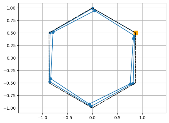
As expected, we can observe some numerical error of the time-scheme, since we do not retrieve exactly the hexagon showed by the exact solution. One accuracy indicator is the \(L_\infty\) error in time (computed over all time-steps) :
[4]:
print("L_inf error : {:1.5f}".format(np.linalg.norm(uNum-uExact, ord=np.inf)))
L_inf error : 0.11925
Now let say we want to use a collocation method instead of RK4, using \(4\) Legendre Radau-II nodes (i.e Radau nodes including the right time interval bound). The only line we have to change in the previous code is :
[5]:
# replace : "rk = Q_GENERATORS["RK4"]()" by
coll = Q_GENERATORS["coll"](nNodes=4, nodeType="LEGENDRE", quadType="RADAU-RIGHT")
Then the exact same code as before can be used to build the time-stepper, compute the numerical solution and the error. In practice, you don’t have to, as the \(Q\)-generators in qmat already provides dedicated methods for that :
[6]:
uNum = coll.solveDahlquist(lam, u0, tEnd, nSteps)
plt.plot(uNum[0].real, uNum[0].imag, 's', ms=10, c="orange")
plt.plot(uNum.real, uNum.imag, 'o-')
plt.axis("equal")
plt.grid()
print("L_inf error : {:1.5f}".format(coll.errorDahlquist(lam, u0, tEnd, nSteps, uNum=uNum)))
L_inf error : 0.00001

Now the error is way lower, even if we used \(Q\)-coefficients of the same size … but there is a major difference here between the two \(Q\) matrices :
[7]:
print("Q for RK4 :")
print(rk.Q)

print("Q for Collocation :")
print(coll.Q)
Q for RK4 :
[[0.  0.  0.  0. ]
 [0.5 0.  0.  0. ]
 [0.  0.5 0.  0. ]
 [0.  0.  1.  0. ]]
Q for Collocation :
[[ 0.11299948 -0.04030922  0.02580238 -0.00990468]
 [ 0.234384    0.20689257 -0.04785713  0.01604742]
 [ 0.21668178  0.40612326  0.18903652 -0.0241821 ]
 [ 0.22046221  0.38819347  0.32884432  0.0625    ]]
While \(Q\) is dense for the collocation method, it is lower triangular for RK4, which allows to solve for the first node (or stage) first, then the second one, etc … Hence we need to solve instead \(M\) equations sequentially instead of solving a system of \(M\) equations all-at-once, reducing thus the computation cost for one time-step. This is one reason why RK methods have been generally favored in scientific computing against collocation methods.
🔍 In this case (Dahlquist), solving the all-at-once system is easy and cheap as showed above. But for large scale non-linear problems, this can quickly become unfeasible, as solution at each time node may represent thousands or millions of degrees of freedom …
However, the high accuracy of collocation methods motivates to solve the all-at-once system in a cheaper way, which is the main idea of Spectral Deferred Correction (SDC), a.k.a Iterated Runge-Kutta methods. Those use fixed-point preconditioned iterations to solve the all-at-once system, where the preconditoner is built using a lower triangular approximation of the \(Q\) matrix, named the \(Q_\Delta\) matrix.
The second main feature of qmat is then to generate those approximations …