Tutorial 2 : using the qmat.nodes module

📜 The NodeGenerator class from qmat.nodes allows to generate sets of quadrature nodes associated to various types of orthogonal polynomials. It is based on the book of W. Gautschi :Orthogonal Polynomials: Computation and Approximation.

Gauss quadrature approximate integrals by a given quadrature rule on \(M\) points :

\[\int_{-1}^{1} f(t)\omega(t)dt \simeq \sum_{m=1}^{M} \omega^M_m f(\tau^M_m)\]

where \(f(t)\) is a function of interest, \(\omega(t)\) a weight function and \(\tau^M_m, \omega^M_m\) are the quadrature nodes and weights associated to the Gauss quadrature on \(M\) points. In particular, the quadrature nodes \(\tau^M_m\) are the roots a given polynomial belonging to an orthogonal basis with respect to the scalar product :

\[\langle p,q \rangle = \int_{-1}^{1} p(t)q(t) \omega(t)dt\]

This polynomial basis is solely determined by the weights function \(\omega(t)\), and classical polynomial basis exist already in the literature :

• \(\omega(t) = 1\) : Legendre polynomials

• \(\omega(t) = \frac{1}{\sqrt{1-t^2}}\) : Chebyshev polynomials of the 1st kind

• \(\omega(t) = \sqrt{1-t^2}\) : Chebyshev polynomials of the 2nd kind

• \(\omega(t) = \frac{\sqrt{1+t^2}}{\sqrt{1-t^2}}\) : Chebyshev polynomials of the 3rd kind

• \(\omega(t) = \frac{\sqrt{1-t^2}}{\sqrt{1+t^2}}\) : Chebyshev polynomials of the 4th kind

Node generation

The type of polynomial defines a node type, and the roots of the \(M^{th}\) degree polynomial of this type are then the quadrature nodes \(\tau^M_m\) and can be generated, e.g for \(M=4\) :

from qmat.nodes import NodesGenerator

gen = NodesGenerator(nodeType="LEGENDRE", quadType="GAUSS")
nodes = gen.getNodes(nNodes=4)
print(nodes)

[-0.86113631 -0.33998104  0.33998104  0.86113631]

💡 Note that those nodes symmetrically distributed, which is not necessarily the case for other types of nodes e.g for the Chebyshev polynomials of the fourth kind :

gen = NodesGenerator(nodeType="CHEBY-4", quadType="GAUSS")
nodes = gen.getNodes(nNodes=4)
print(nodes)

[-0.93969262 -0.5         0.17364818  0.76604444]

Different types of nodes are available, checkout qmat.nodes.NODE_TYPES for the current list, in particular :

• LEGENDRE : for Legendre polynomials

• CHEBY-1 : for the Chebyshev polynomials of the first kind

• CHEBY-2 : …

💡 You may noticed that those nodes are always strictly included in \([-1,1]\), hence usually named Gauss points. But four specific quadrature types can be considered for each node type (i.e for each polynomial basis) :

• GAUSS : nodes do not include \(-1\) or \(1\),

• LOBATTO : nodes include \(-1\) and \(1\),

• RADAU-LEFT : nodes include \(-1\) (usually called Radau-I),

• RADAU-RIGHT : nodes include \(1\) (usually called Radau-II).

The quadrature type is selected when instantiating the node generator, as for the node type :

gen = NodesGenerator(nodeType="LEGENDRE", quadType="LOBATTO")   # usually called Gauss-Lobatto in the literature
nodes = gen.getNodes(nNodes=4)
print(nodes)

[-1.        -0.4472136  0.4472136  1.       ]

gen = NodesGenerator(nodeType="CHEBY-3", quadType="RADAU-LEFT")
nodes = gen.getNodes(nNodes=4)
print(nodes)

[-1.         -0.42720716  0.36290645  0.92144357]

📣 We use the naming convention RADAU-RIGHT / RADAU-LEFT as it is more explicit than the usual one in the literature, and also because Radau-I and Radau-II nodes are usually associated to the Legendre polynomials.

Orthogonal polynomials

The node computation process relies on the three term recurrence coefficients associated to each polynomial basis :

\[\begin{split}\begin{gather} \forall j \in \mathbb{N}, \quad \pi_{j+1}(t) = (t-\alpha_j)\pi_{j}(t) - \beta_j \pi_{j-1}(t), \\ \pi_{-1}(t) = 0, \quad \pi_0(t) = 1. \end{gather}\end{split}\]

Those coefficients are know analytically for each polynomial basis (i.e node type), and are used to generate the tri-diagonal Jacobi matrix for the weight function \(\omega\)

\[\begin{split}J_\infty^{\omega} = \begin{bmatrix} \alpha_0 & \sqrt{\beta_1} & & & \\ \sqrt{\beta_1} & \alpha_1 & \sqrt{\beta_2} & & \\ & \sqrt{\beta_2} & \alpha_2 & \sqrt{\beta_2} & \\ & & \ddots & \ddots & \ddots \end{bmatrix}.\end{split}\]

Computing the eigenvalues of the leading principal sub-matrix of size \(M\) allows to retrieve the GAUSS nodes, and some small modifications of this sub-matrix allow to retrieve the LOBATTO, RADAU-LEFT and RADAU-RIGHT nodes.

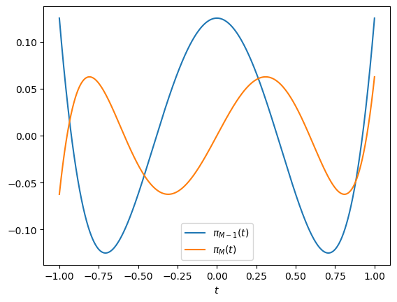
But one can also use the orthogonal coefficients to evaluate the orthogonal polynomial of any degree, e.g for \(M=5\) :

import numpy as np
import matplotlib.pyplot as plt

degree = 4

t = np.linspace(-1, 1, num=10000)

gen = NodesGenerator("CHEBY-1")
alpha, beta = gen.getOrthogPolyCoefficients(degree+1)

pi1, pi2 = gen.evalOrthogPoly(t, alpha, beta)

plt.plot(t, pi1, label=r"$\pi_{M-1}(t)$")
plt.plot(t, pi2, label=r"$\pi_{M}(t)$")
plt.legend(); plt.xlabel("$t$");

📣 Note that the quadType argument does not matter when generating orthogonal polynomials, and can simply be left to its default value.